Visualize your data with charts in Google Sites

Ever since we launched the chart editor in Google spreadsheets, many of you have asked us to integrate charts into Google Sites as well. Today we are making this possible. Now you can display charts in your Sites by going to Insert Menu and choosing Charts in edit mode.

Once you select a spreadsheet, the editor picks existing charts from the spreadsheet to embed into a Site.

You can also create a chart by specifying the sheet and range and customize the chart by changing various properties such as color, axes, labels and more. Choose which chart type best expresses your data or let the chart editor recommend one for you.

You can decide to choose between two modes Live and Snapshot to show the data.

• Live provides you with dynamic charts. Whenever the chart is loaded in the Site, the chart will display the most recent data in the spreadsheet. This is very useful in cases when the spreadsheet data is updated manually or using a script.


• Snapshot means just that. It’s a snapshot at a point in time, so the chart will store and display the exact same data, regardless of whether you make changes to the underlying data sheet.

Changes made to charts in Sites are independent to the specific chart, so the same spreadsheet data can be applied across multiple charts.

To learn more about how to express your data more visually with Sites, visit the help center. Be sure to let us know what you think in the comments.

Posted by: Hillel Maoz, Software Engineer

Trying on the new Dynamic Views from Blogger

As you may have noticed, the Docs blog looks a lot different today. That’s because we—along with a few other Google blogs—are trying out a new set of Blogger templates called Dynamic Views.

Launched today, Dynamic Views is a unique browsing experience that makes it easier and faster for readers to explore blogs in interactive ways. We’re using the Classic view, but you can also preview this blog in any of the other six new views by using the view selection bar at the top left of the screen.



We’re eager to hear what you think about the new Dynamic Views. You can submit feedback using the “Send feedback” link on the bottom right of this page.

If you like what you see here, and we hope you do, we encourage you to try out the new look(s) on your own blog—read the Blogger Buzz post for more info.

Posted by Meredith Blackwell, Google Docs Marketing Manager

This week in Docs: Import/export and paste special improvements

Yesterday, we announced the vertical merge feature in Google spreadsheets, and today we’re happy to share two new features that we hope will make analyzing data a little more efficient.

More import and export support in Google spreadsheets
Now you can convert most pivot tables between Microsoft Excel files and Google spreadsheets for powerful data analysis in whatever file format you prefer. Additionally, filters that help you better visualize and organize your data are now supported in our import and export conversion tools.

To import a pivot table you created in Microsoft Excel, click the File menu in Google spreadsheets, and select import, then select the file from the import options, and click the import button. If you’ve created a pivot table in Google spreadsheets, go to File in the spreadsheet, then click Download As, and choose Excel.

More paste special options in Google spreadsheets
Sometimes you need to copy data in cells that have lots of formatting and formulas, but you don’t always want to paste everything in the cell. For instance, you may want to copy and paste the data in a range of cells, but not the borders that you placed around the cells.

We’ve added four new paste special options including: paste all cell contents except borders, formulas only, data validation only, or conditional formatting only. You can find these new options in a list under “Paste Special” in the Edit menu of Google spreadsheets.


We hope these latest features make working with Google spreadsheets more efficient and productive. As always, let us know what you think in the forum or in the comments.

Posted by: Dan Gundrum, Product Manager

Merge cells vertically in Google spreadsheets

There are many times when you want to format your spreadsheets in a certain way to make your data easier to read and understand. Starting today, we’ve extended the merge functionality to let you create vertical merges across several rows of data.

In the spirit of the NFL season, let’s say you want to host a football tournament for your friends. To make it easier for them to cast their votes on the winning team, you organize the NFL teams by conference and division in a Google spreadsheet. Using vertical merges, you can assign headers to sets of rows. Simply select the set of cells you’d like to merge, then click on the down arrow next to the merge icon, and select Merge vertically.


In the NFL spreadsheet, you’ll see that some of the team names don’t fit on one line in the width of the cells of Column C.

To improve the formatting, select the cells across all the rows of teams in the AFC (rows 2-17) and 2 columns (C and D) and click Merge horizontally. You’ll have 16 merged cells that span 2 columns for better formatting.


After applying vertical merges to all of the conference and division headers and horizontal merges across the team names in each conference, you’re ready to share with your friends for the tournament!


To undo a merge action, select a merged cell and click Unmerge in the drop-down menu.

We hope you enjoy customizing the formatting of your spreadsheets with this feature. Let us know what you think in the comments.

Posted by: Jakov Krolo, Software Engineer Intern

+1 button in Google Sites

We have been thrilled with the response to the launch of the +1 button on websites all across the web, but we also heard that you’d like a simple way to add the +1 button to your own Google Sites. Adding the +1 button to your site will allow your visitors to recommend it to their friends and contacts, which helps more people discover it via their personalized search results.

Starting today, you can add the +1 button to any individual page by choosing +1 Button from the Insert menu, or you can add it to your site’s sidebar and have it appear on every page instantly by editing your Site Layout under Manage Site.


Try it out and let us know what you think in the forum.

Posted by: Michael Verrilli, Software Engineer

Improved Accessibility in Google Docs and Sites

Today we announced some of the updates we’ve released recently to make Google’s applications more accessible to the blind community. For Google Docs and Sites, we’re pleased to announce new keyboard shortcuts and better screen reader support for our blind users.

Screen reader support in Google Docs and Sites
To help blind users read, edit and navigate content, Google Docs (including documents list, documents and spreadsheets) and Sites now support two screen readers: JAWS and ChromeVox. Here are a few examples of how screen readers work in Google Docs and Sites:

• In documents, you’ll hear feedback when you format text or insert tables, lists or comments in your document.
  
• In spreadsheets, you’ll hear the cell’s location, contents and comments when moving between cells.
  
• In both documents and spreadsheets, you’ll hear feedback as you navigate to areas outside the main content area, such as the menu bar, chat pane and dialog boxes.
  
• In your documents list, you’ll hear feedback when you upload or download a file, organize collections or move between files in your documents list.
  
• In Sites, you’ll hear feedback as you navigate and manage your sites, create and edit pages, and navigate through menus and dialog boxes.

For a complete list of screen reader-supported features and instructions for how to use them, visit the Docs and Sites help centers.

New keyboard shortcuts
We’ve also added new keyboard shortcuts to make it easier to use Google Docs and Sites. In your documents list, for example, you can use the up and down arrow keys to move through the files in the list, and you can open the selected document by hitting Enter. For a complete list of keyboard shortcuts, please refer to the help center articles for spreadsheets, documents, documents list and Sites.

With these new accessibility features, we hope to make it easier for everyone to use Google Docs and Sites. Please use this form to share your feedback directly with the accessibility team so we can continue to improve our products.

Posted by: Jeff Harris, Product Manager

This week in Docs: Format painter, Google Fusion Tables, and drag & drop images

This week in Docs, we’re introducing three new tools that put the fun in functional.

Format painter in Google documents

First, we’ve added a format painter to help you copy formatting within Google documents. The new format painter allows you to copy the style of your text, including font, size, color and other formatting options and apply it somewhere else in your document. To use the format painter, select the text for the formatting you want to copy, press the paintbrush button in your toolbar, and then select the text where you want to apply that formatting.

If you double-click on the format painter icon, you’ll enter a mode that lets you select multiple sections of text so you can apply the same formatting to each section.

You can also use keyboard shortcuts for format painting. To copy the style of your selected text, press Ctrl+Option+C for Mac or Ctrl+Alt+C for Windows. To apply any copied styles to whatever text you have selected, press Ctrl+Option+V for Mac or Ctrl+Alt+V for Windows.

Google Fusion Tables in documents list

With this week’s update, we’re also integrating Google Fusion Tables into your documents list. Google Fusion Tables is a data management web application that makes it easy to gather, visualize and collaborate on data online. Now you’ll be able to store and share your Fusion Tables with the rest of the files in your documents list.

Recently, people have used Google Fusion Tables to:

• Visualize evacuation zones for New York City during Hurricane Irene
  
• Host data sets made public by the State of California
  
• Gather data from local flu shot clinics for Google Flu Vaccine Finder
  
• Map shelters and road status during the tsunami crisis in Japan

Go to Create new > Table from your documents list menu to get started visualizing or sharing tables of data in .csv, .xls or .kml files.

We're working on making Google Fusion Tables available to Google Apps customers and will let you know as soon as they are. Take a tour to learn more about Google Fusion Tables.

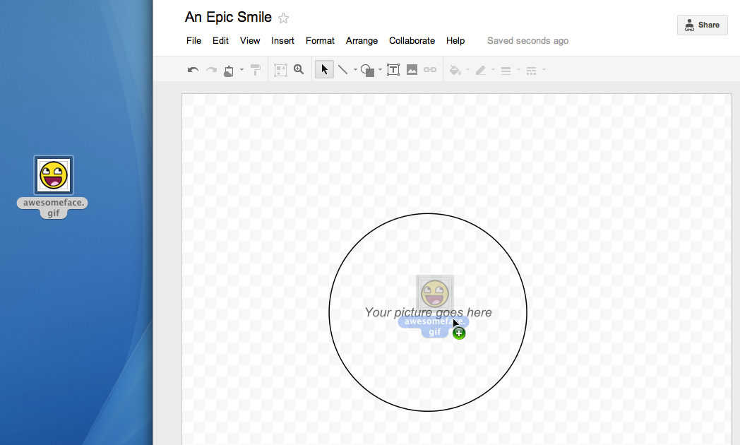
Drag & drop images in Google drawings

We also made it easier to add images from your desktop to Google drawings. If you’re using the latest version of Chrome, Safari, or Firefox, you can now drag an image from your desktop and drop it directly in the drawing canvas.


Give these tools a try and let us know what you think in the comments.

Posted by: Micah Lemonick, Software Engineer

Updated 9/13 to add shortcuts for Windows

Comment-only access in Google documents

In the past several months, we’ve added new discussion and commenting features to improve collaboration in Google documents. As an engineer, I often create docs with design concepts and send them to my team to review and provide feedback, and we use the commenting features to facilitate these discussions. Sometimes, I want to let team members view and make comments without allowing them to directly edit my document.

Over the next several days, we're releasing a new sharing option so that you can let people view and add comments to your documents without giving them edit access. To give comment-only access to your document, click on the Share button. From there, add in the contact you’d like to share your document with, and select Can comment.


You can also choose to give comment-only access to anyone with the link or anyone on the web by changing the sharing settings within the document. To do this, click Change in the sharing settings window and change visibility options to Public on the web or Anyone with the link, then change the access options to Can comment.

Similarly, if you’re using a Google Apps account, click Change in the sharing settings and select either “People at [your domain] who have the link can access” or “People at [your domain] can find and access.” Then change access option to Can comment.


Users that have comment-only access can view your document and add comments throughout -- without being able to change the content of the document directly.

We hope this latest feature in discussions helps you get the feedback you need while providing you with more control over the content in your docs. So comment away and tell us what you think -- below or in the forum.

Posted by: Sarah Wu, Software Engineer

What Happened Wednesday

Not our best week. On Wednesday we had an outage that lasted one hour and meant that document lists, documents, drawings and Apps Scripts were inaccessible for the majority of our users. We use Google Docs ourselves every day, so we feel your pain and are very sorry.

So what happened? The outage was caused by a change designed to improve real time collaboration within the document list. Unfortunately this change exposed a memory management bug which was only evident under heavy usage.

Every time a Google Doc is modified, a machine looks up the servers that need to be updated. Due to the memory management bug, the lookup machines didn’t recycle their memory properly after each lookup, causing them to eventually run out of memory and restart. While they restarted, their load was picked up by the remaining lookup machines - making them run out of memory even faster. This meant that eventually the servers couldn’t properly process a large fraction of the requests to access document lists, documents, drawings, and scripts which led to the outage you saw on Wednesday.

Our automated monitoring noticed that attempts to access documents were failing at an increased rate, and alerted us 60 seconds later after the failure rate increased sharply. The engineering teams diagnosed the problem, determined that it was correlated with the feature change, and started rolling it back 23 minutes after the first alert. In parallel, we doubled the capacity of the lookup service to mitigate the impact of the memory management bug. The rollback completed 24 minutes later, and 5 minutes after that the outage was effectively over as the additional capacity restored normal function.

Since resolution, we have been assembling and scrutinizing the timeline of this event, and have assembled a list of steps which will both reduce the chance of a future event, decrease the time required to notice and resolve a problem, and limit the scope which any single problem can affect. We intend to take all these steps; some are not easy, but we're committed to keeping Google's services exceptionally reliable. In the meantime, rest assured that we take every outage very very seriously, and as always we'll post a full incident report of what happened to the Apps Dashboard once our investigation is complete. Again, we apologize for the inconvenience and frustration which the outage has caused.

Posted by: Alan Warren, Engineering Director

Tips & Tricks: Using the new Subtotal function in Google spreadsheets

This week, we added the Subtotal function to our list of functions in Google spreadsheets. One of the benefits of the Subtotal function is that it works well with AutoFilters by only using unfiltered data when performing calculations (other functions such as Sum include filtered data calculations). Subtotal also lets you change what function you’re performing on those values very quickly, by selecting an item from a drop-down list. See our help article for details.

This versatile function is often used by accountants, finance professionals, and business consultants. It can also be extremely convenient for any user -- let’s show you why.



Say that you’re helping to plan your family’s annual Labor Day beach weekend. You want to decide how many hot dogs and veggie dogs to buy. To figure this out, you create a Google spreadsheet that includes all your family members, their meat preferences, and the number of hot dogs everyone ate at the past several family gatherings:

To quickly count how many veggie dogs you need to buy based off the number of veggie dogs eaten last month, add a filter to the columns , sort to “Yes” only in Column C, and type in this Subtotal function underneath the table:

=SUBTOTAL(109, F2:F14)



Cells F2 through F14 show the number of hot dogs each family member ate last month. “109” is the code that references the Sum function (“9” would also work). Typing in a regular Sum function in this case (=SUM(F2:F14)) would have added all dogs, veggie or not, whereas Subtotal ignores hodogs which have been filtered.

Another neat feature of the Subtotal function is that the function code (such as “109” above) can easily be changed to refer to different operations like Average, Minimum, and Maximum. As a result, Subtotal can be used to condense a number of calculations into a small space.



Let’s say you want to see not only the total number of hot dogs eaten each summer month, but also the average number eaten. Rather than creating two different functions (Sum and Average) for each month, you can use Subtotal.

• In an open cell -- let’s use B15 -- you would create a drop-down list with the codes for the Sum and Average function (109 and 101 respectively).
• And under the column for each month, you would write a Subtotal function, but reference cell B15 instead of typing in a code.

For June, therefore, your function would read: =SUBTOTAL(B15, D2:D14)



Every time you change which code appears in cell B15 through the drop-down, the values under each month will change, showing either the total or the average number of hot dogs eaten by your family with just one click.





We hope the Subtotal function makes your data analysis a lot easier -- and maybe even more fun.



Posted by: Lai Kwan Wong, Software Engineer